You can find the source code for this file in the class repository. The direct link is here.

Model

Let’s start with studying static labor supply. We will consider the decision of the agent under the following rule:

\[ \max_{c,h} \frac{c^{1+\eta}}{1+\eta} - \beta \frac{h^{1+\gamma}}{1+\gamma}\\ \text{s.t. } c = \rho \cdot w\cdot h -r + \mu - \beta_0 \cdot 1[h>0] \\ \] The individual takes his wage \(w\) as given, he chooses hours of work \(h\) and consumption \(c\) subject to a given non labor income \(\mu\) as well as a tax regime defined by \(\rho,r\). \(\beta_0\) is a fixed cost associated with working. We ignore participation here, see the homework for including it.

We note already that the non labor income can control for dynamic labor supply since we can have \(\mu= b_t - (1+r)b_{t+1}\). This is part of a larger maximization problem where the agents choose optimaly \(b_t\) over time. We will get there next time.

Finding solution

The first order conditions give us \(w(wh +r - \mu)^\eta = \beta h^\gamma\). There is no closed-form but we can very quickly find an interior solution by using Newton maximization on the function \(f(x) = w(wh +r - \mu)^\eta - \beta h^\gamma\). We iterate on

\[x \leftarrow x - f(x)/f'(x).\]

# function which updates choice of hours using Newton step
# R here is total unearned income (including taxes when not working and all)
ff.newt <- function(x,w,R,eta,gamma,beta) {
  f0 = w*(w*x + R)^eta - beta*x^gamma
  f1 =  eta*w^2 * (w*x + R)^(eta-1) - gamma * beta *x^(gamma-1)
  x  = x - f0/f1 
  x  = ifelse(w*x + R<=0, -R/w + 0.0001,x) # make sure we do not step out of bounds for next iteration
  x  = ifelse(x<0, 0.0001,x)
  x
}

Simulating data

We are going to simulate a data set where agents will choose participation as well as the number of hours if they decide to work. To do that we will solve for the interior solution under a given tax rate and compare this to the option of no-work.

p  = list(eta=-1.5,gamma = 0.8,beta=1,nu=0.5) # define preferences
tx = list(rho=1,r=0) # define a simple tax
N=50000
simdata = data.table(i=1:N,X=rnorm(N))
simdata <- simdata[,lw := X     + rnorm(N)*0.2];      # add a wage which depends on X
simdata <- simdata[,mu := exp(0.3*X + rnorm(N)*0.2)]; # add non-labor income that also depends on X

# we then solve for the choice of hours and consumption
simdata <- simdata[, h := pmax(-mu+tx$r ,0)/exp(lw)+1] # starting value
# for loop for newton method (30 should be enough, it is fast)
for (i in 1:30) {
  simdata[, h := ff.newt(h,tx$rho*exp(lw),mu-tx$r,p$eta,p$gamma,p$beta) ]
}

# attach consumption, value of working
simdata <- simdata[, c  := tx$rho*exp(lw)*h + mu];
simdata <- simdata[, u1 := c^(1+p$eta)/(1+p$eta) - p$beta * h^(1+p$gamma)/(1+p$gamma) ];

At this point we can regress \(\log(w)\) on \(\log(c)\) and \(\log(h)\) and find precisely the parameters of labor supply:

pander(summary(simdata[,lm(lw ~ log(c) + log(h))]))

## Warning in summary.lm(simdata[, lm(lw ~ log(c) + log(h))]): essentially perfect
## fit: summary may be unreliable

	Estimate	Std. Error	t value
(Intercept)	5.084e-16	7.772e-18	65.42
log(c)	1.5	4.014e-18	3.737e+17
log(h)	0.8	7.601e-18	1.053e+17

Fitting linear model: lw ~ log(c) + log(h)
Observations	Residual Std. Error	\(R^2\)	Adjusted \(R^2\)
50000	4.589e-16	1	1

The regression still works, among each individual who chooses to work, the FOC is still satisfied.

Heterogeneity in \(\beta\)

Finally we want to add heterogeneity in the \(\beta\) parameter.

simdata <- simdata[,betai := exp(p$beta*X+rnorm(N)*0.1)]
simdata <- simdata[, h := pmax(-mu+tx$r ,0)/exp(lw)+1]
for (i in 1:30) {
  simdata <- simdata[, h := ff.newt(h,tx$rho*exp(lw),mu-tx$r,p$eta,p$gamma,betai) ]
}

# attach consumption
simdata <- simdata[, c  := exp(lw)*h + mu];

# let's check that the FOC holds
sfit = summary(simdata[,lm(lw ~ log(c) + log(h) + log(betai))])

## Warning in summary.lm(simdata[, lm(lw ~ log(c) + log(h) + log(betai))]):
## essentially perfect fit: summary may be unreliable

expect_equivalent(sfit$r.squared,1)
expect_equivalent(coef(sfit)["log(c)",1],-p$eta)
expect_equivalent(coef(sfit)["log(h)",1],p$gamma)

# omitting betai doesn't work 
sfit2 = summary(simdata[,lm(lw ~ log(c) + log(h))])
expect_false(coef(sfit2)["log(c)",1]==-p$eta)

# finally we can try a natural regression since we don't observe betai directly:
sfit3 = summary(simdata[,lm(lw ~ log(c) + log(h) + X)])

pander(sfit3)

	Estimate	Std. Error	t value
(Intercept)	-0.07707	0.001806	-42.66
log(c)	1.278	0.003141	407
log(h)	0.5794	0.001985	291.9
X	0.938	0.001469	638.5

Fitting linear model: lw ~ log(c) + log(h) + X
Observations	Residual Std. Error	\(R^2\)	Adjusted \(R^2\)
50000	0.08738	0.9926	0.9926

Simple case of \(\eta=0\)

p  = list(eta=0,gamma = 0.8,beta=1,beta0=0,nu=0.5) # define preferences
tx = list(rho=1,r=0) # define a simple tax
N=500
simdata = data.table(i=1:N,X=rnorm(N))
simdata <- simdata[,lw := X     + rnorm(N)*0.2];      # add a wage which depends on X
simdata <- simdata[,mu := exp(0.3*X + rnorm(N)*0.2)]; # add non-labor income that also depends on X
simdata <- simdata[,eps := rnorm(N)*0.1]
simdata <- simdata[,betai := exp(p$nu*X+eps)]
simdata <- simdata[, h := (tx$rho*exp(lw)/betai)^(1/p$gamma)]

sfit3 = summary(simdata[,lm(log(h) ~ lw + X)])
pander(sfit3)

	Estimate	Std. Error	t value	Pr(>\|t\|)
(Intercept)	-0.008012	0.005659	-1.416	0.1575
lw	1.292	0.0274	47.17	1.227e-185
X	-0.6619	0.02791	-23.72	1.001e-83

Fitting linear model: log(h) ~ lw + X
Observations	Residual Std. Error	\(R^2\)	Adjusted \(R^2\)
500	0.1264	0.9673	0.9672

sfit4 = summary(simdata[,lm(lw ~ log(h) + X)])
pander(sfit4)

	Estimate	Std. Error	t value	Pr(>\|t\|)
(Intercept)	0.004599	0.003962	1.161	0.2462
log(h)	0.6325	0.01341	47.17	1.227e-185
X	0.6008	0.009286	64.7	3.091e-244

Fitting linear model: lw ~ log(h) + X
Observations	Residual Std. Error	\(R^2\)	Adjusted \(R^2\)
500	0.08839	0.9926	0.9926

Then we can construct a counter-factual revenue

p2  = list(eta=0,gamma = 1/sfit3$coefficients["lw","Estimate"],beta=1,beta0=0)
tx2 = tx
tx2$rho = 0.9
simdata <- simdata[, h2 := (tx2$rho*exp(lw)/betai)^(1/p2$gamma)]

simdata[, list(totearnings =mean(exp(lw+h)), R1=mean((1-tx$rho)*exp(lw+h)),R2=mean((1-tx2$rho)*exp(lw+h2)) ,R3=mean((1-tx2$rho)*exp(lw+h)) )]

##    totearnings R1       R2       R3
## 1:    421.1042  0 25.39596 42.11042

Heterogeneity in \(\beta\) revisited

Finally we want to add heterogeneity in the \(\beta\) parameter.

p  = list(eta=-1.5,gamma = 0.8,beta=1,beta0=0,nu=0.5) # define preferences
tx = list(rho=1,r=0) # define a simple tax
N=5000
simdata = data.table(i=1:N,X=rnorm(N))
simdata <- simdata[,lw := X     + rnorm(N)*0.2];      # add a wage which depends on X
simdata <- simdata[,mu := exp(0.3*X + rnorm(N)*0.2)]; # add non-labor income that also depends on X
simdata <- simdata[,eps := rnorm(N)*0.1]
simdata <- simdata[,betai := exp(p$nu*X+eps)]
simdata <- simdata[, h := (tx$rho*exp(lw)/betai)^(1/p$gamma)]
simdata <- simdata[, betai := exp(p$nu*X+rnorm(N)*0.1)]
simdata <- simdata[, h := pmax(-mu+tx$r ,0)/exp(lw)+1]
for (i in 1:30) {
  simdata <- simdata[, h := ff.newt(h,tx$rho*exp(lw),mu-tx$r,p$eta,p$gamma,betai) ]
}

# attach consumption
simdata <- simdata[, c  := exp(lw)*h + mu];

# let's check that the FOC holds
sfit = summary(simdata[,lm(lw ~ log(c) + log(h) + log(betai))])

## Warning in summary.lm(simdata[, lm(lw ~ log(c) + log(h) + log(betai))]):
## essentially perfect fit: summary may be unreliable

expect_equivalent(sfit$r.squared,1)
expect_equivalent(coef(sfit)["log(c)",1],-p$eta)
expect_equivalent(coef(sfit)["log(h)",1],p$gamma)

sfit2 = summary(simdata[,lm(lw ~ log(c) + log(h))])
expect_false(coef(sfit2)["log(c)",1]==-p$eta)

sfit3 = summary(simdata[,lm(lw ~ log(c) + log(h) + X)])

pander(sfit2)

	Estimate	Std. Error	t value
(Intercept)	-0.5719	0.007982	-71.65
log(c)	2.413	0.008067	299.2
log(h)	0.5701	0.0123	46.34

Fitting linear model: lw ~ log(c) + log(h)
Observations	Residual Std. Error	\(R^2\)	Adjusted \(R^2\)
5000	0.1802	0.9692	0.9692

Next we have established the following condition in the class:

\[ E \left[ \log(w) - \gamma \log h - \eta \log c + \nu x | W,R,X \right] = 0 \] This suggests an IV strategy where we instrument using \(W,R,X\). We can use either hours or consumption as a dependent variable and instrument the other. We use \(h\) and implement using 2SLS (identical to IV in this case). We then first regress \(c\) on the three variables to get the predicted component, that we then use in a regression.

fit_c = simdata[, lm( log(c) ~ lw + log(mu) + X ) ]
simdata[, c_iv := predict(fit_c)]

sfit_iv2 = simdata[, lm( log(h) ~ c_iv + lw +  X   )]

pander(sfit_iv2)

Fitting linear model: log(h) ~ c_iv + lw + X
	Estimate	Std. Error	t value	Pr(>\|t\|)
(Intercept)	0.02051	0.007676	2.672	0.007572
c_iv	-1.92	0.01774	-108.2	0
lw	1.272	0.01095	116.1	0
X	-0.6286	0.007817	-80.42	0

Where we find as regression coefficients \(1/\gamma\) and \(\eta/\gamma\). Note of course that the inference out of the second regression is no valid (need to use IB formula, not only the second stage).

fit_c = simdata[, lm( log(c) ~ lw + log(mu) + X ) ]
simdata[, c_iv := predict(fit_c)]

sfit_iv2 = simdata[, lm( log(h) ~ c_iv + lw +  X   )]

pander(sfit_iv2)

Fitting linear model: log(h) ~ c_iv + lw + X
	Estimate	Std. Error	t value	Pr(>\|t\|)
(Intercept)	0.02051	0.007676	2.672	0.007572
c_iv	-1.92	0.01774	-108.2	0
lw	1.272	0.01095	116.1	0
X	-0.6286	0.007817	-80.42	0

Heckman selection

We cover here a simple version of the Heckman selection. In the labor supply homework, you will see a version of this closer to the structure of the model presented at the begining of this page.

We start with the following model:

\[ \begin{align} y_i^* & = \gamma x_i + \epsilon_i \\ d_i & = 1[ \delta_1 x_i + \delta_2 z_i + u_i \geq 0] \\ y_i & = d_i \cdot y_i^* \end{align} \] And only \((y_i, d_i, x_i, z_i)\) are observed. We assume that \((\epsilon_i,u_i)\) are jointly normal, mean zero and independent of \(x_i\).

N=5000
p = list(gamma = 1.0, delta1 = 0.8, delta2 = 0.8, alpha = 1.0, sigma_v = 1.0, sigma_u = 1.0)
X = 2*runif(N)-1
Z = 2*runif(N)-1
U = p$sigma_u * rnorm(N)
D = p$delta1 * X + p$delta2 * Z + U >= 0 
E = p$alpha * U + p$sigma_v * rnorm(N)
Ys = p$gamma * X + E 

data = data.table(y = Ys * D, ys=Ys, d = D, x=X,z=Z,e=E,u=U)
data[ d==FALSE, y:=NA]

While \(E[ \epsilon_i | x_i ]=0\) we can’t use that for identification since what we observe is \((y_i, x_i)\) and note \((y^*_i, x_i)\), so we can’t construct \(E[ y^*_i x_i ]\).

We then need to rely on something else. We are going to look at \(E[ y^*_i x_i | d_i \geq 0 ]\) which is then equal to \(E[y_i x_i | d_i \geq 0 ]\) which is observed!

fit1 = lm(y ~ x,data)
summary(fit1)

## 
## Call:
## lm(formula = y ~ x, data = data)
## 
## Residuals:
##     Min      1Q  Median      3Q     Max 
## -3.6667 -0.8478 -0.0356  0.8562  4.3819 
## 
## Coefficients:
##             Estimate Std. Error t value Pr(>|t|)    
## (Intercept)  0.69628    0.02647   26.30   <2e-16 ***
## x            0.67998    0.04649   14.62   <2e-16 ***
## ---
## Signif. codes:  0 '***' 0.001 '**' 0.01 '*' 0.05 '.' 0.1 ' ' 1
## 
## Residual standard error: 1.235 on 2494 degrees of freedom
##   (2504 observations deleted due to missingness)
## Multiple R-squared:  0.07899,    Adjusted R-squared:  0.07862 
## F-statistic: 213.9 on 1 and 2494 DF,  p-value: < 2.2e-16

We we compare the regression coefficient 0.6799819 to the true parameter 1. We can look at the distribution of the error.

#ggplot(data, aes(x = x, y= e)) + geom_smooth() + 
#  theme_bw() + geom_hline(yintercept=0,linetype=2)
ggplot(data[d==TRUE], aes(x = x, y= e)) + geom_smooth() + 
  theme_bw() + geom_hline(yintercept=0,linetype=2)

## `geom_smooth()` using method = 'gam' and formula = 'y ~ s(x, bs = "cs")'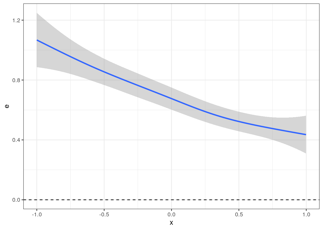

We then look at

\[ \begin{align} E[y_i | x_i, z_i, d_i=1 ] & = E[y^*_i | x_i, z_i, d_i=1 ] \\ & = E[\gamma x_i +\epsilon_i | x_i, z_i, d_i=1 ] \\ & = \gamma x_i + E[\epsilon_i | x_i, z_i, d_i=1 ] \\ \end{align} \] \((\epsilon_i,u_i)\) are jointly normal so we know we can write \(\epsilon_i = \alpha u_i + v_i\) where \(v_i\) is normal, mean zero and independent of \(u_i\). We can then write the conditional expectation as follows:

\[ \begin{align} E[\epsilon_i | x_i, z_i, d_i =1 ] & =E[\epsilon_i | x_i, z_i, \delta_1 x_i + \delta_2 z_i + u_i \geq 0 ] \\ & =E[\alpha u_i + v_i | x_i, z_i, \delta_1 x_i + \delta_2 z_i + u_i \geq 0 ] \\ & = \alpha E[u_i | x_i, z_i, \delta_1 x_i + \delta_2 z_i + u_i \geq 0 ] \\ & \quad \quad \quad \quad + E[v_i | x_i, z_i, \delta_1 x_i + \delta_2 z_i + u_i \geq 0 ] \\ & = \alpha E[u_i | x_i, z_i, \delta_1 x_i + \delta_2 z_i + u_i \geq 0 ] + 0 \\ & = \alpha E[u_i | u_i \geq -\delta_2 z_i -\delta_1 x_i ] \\ \end{align} \] Finally, we note that \(u_i\) is a normal distribution with some variance \(\sigma^2_u\). And we want to compute the mean of that distribution conditional on being lower than some value.

We can look at that.

\[ \begin{align} E[u_i | u_i \geq a ] & = \int_a^{\infty} u f_{u>a}(u) du \\ & = \int_a^{\infty} u \frac{1}{1-\Phi(\frac{a}{\sigma_u})} \frac{1}{\sigma_a} \phi ( \frac{u}{\sigma_u}) du \\ & = \frac{1}{1-\Phi(\frac{a}{\sigma_u})} \int_a^{-\infty} u \frac{1}{\sigma_u \sqrt{2 \pi }} \exp ( - \frac{u^2}{2\sigma_u^2}) du \\ & = \frac{1}{1-\Phi(\frac{a}{\sigma_u})} \Big[ \frac{-\sigma_u}{ \sqrt{2 \pi}} \exp ( - \frac{u^2}{2\sigma_u^2}) \Big]^{\infty}_a \\ & = \sigma_u \frac{ \phi(\frac{a}{\sigma_u})}{1-\Phi(\frac{a}{\sigma_u})} \\ \end{align} \] And so we we have that

\[ \alpha E[u_i | u_i \geq -\delta_2 z_i -\delta_1 x_i] = \alpha \sigma_u \frac{ \phi(\frac{-\delta_2 z_i -\delta_1 x_i}{\sigma_u})}{1-\Phi(\frac{-\delta_2 z_i -\delta_1 x_i}{\sigma_u})} \]

Which means that we need a value for \(\frac{\delta_1}{\sigma_u}\) and \(\frac{\delta_2}{\sigma_u}\). Luckily the participation decision given by \(\delta_2 z_i + \delta_1 x_i + u_i \geq 0\) and so the probit regression of \(d_i\) on \(z_i\) and \(x_i\) gives precisely these coefficients!

Indeed

fit2 = glm(d ~ x + z, family = binomial('probit'), data)
summary(fit2)

## 
## Call:
## glm(formula = d ~ x + z, family = binomial("probit"), data = data)
## 
## Deviance Residuals: 
##     Min       1Q   Median       3Q      Max  
## -2.3630  -0.9623  -0.3386   0.9596   2.4600  
## 
## Coefficients:
##             Estimate Std. Error z value Pr(>|z|)    
## (Intercept) -0.01235    0.01919  -0.643     0.52    
## x            0.83759    0.03493  23.982   <2e-16 ***
## z            0.83712    0.03458  24.210   <2e-16 ***
## ---
## Signif. codes:  0 '***' 0.001 '**' 0.01 '*' 0.05 '.' 0.1 ' ' 1
## 
## (Dispersion parameter for binomial family taken to be 1)
## 
##     Null deviance: 6931.5  on 4999  degrees of freedom
## Residual deviance: 5731.3  on 4997  degrees of freedom
## AIC: 5737.3
## 
## Number of Fisher Scoring iterations: 3

We can then use this to reconstruct our inverse mills ratio. Note that we don’t actually now the coefficient in the front. We don’t need it though.

data[, ai := predict(fit2)]
data[, m := dnorm(ai)/pnorm(ai)]

ggplot(data[d==TRUE], aes(x = x, y= e)) + geom_smooth(se=FALSE) + 
  geom_smooth(aes(y=m),color='red',se=FALSE) + theme_bw() #+ geom_point()

## `geom_smooth()` using method = 'gam' and formula = 'y ~ s(x, bs = "cs")'
## `geom_smooth()` using method = 'gam' and formula = 'y ~ s(x, bs = "cs")'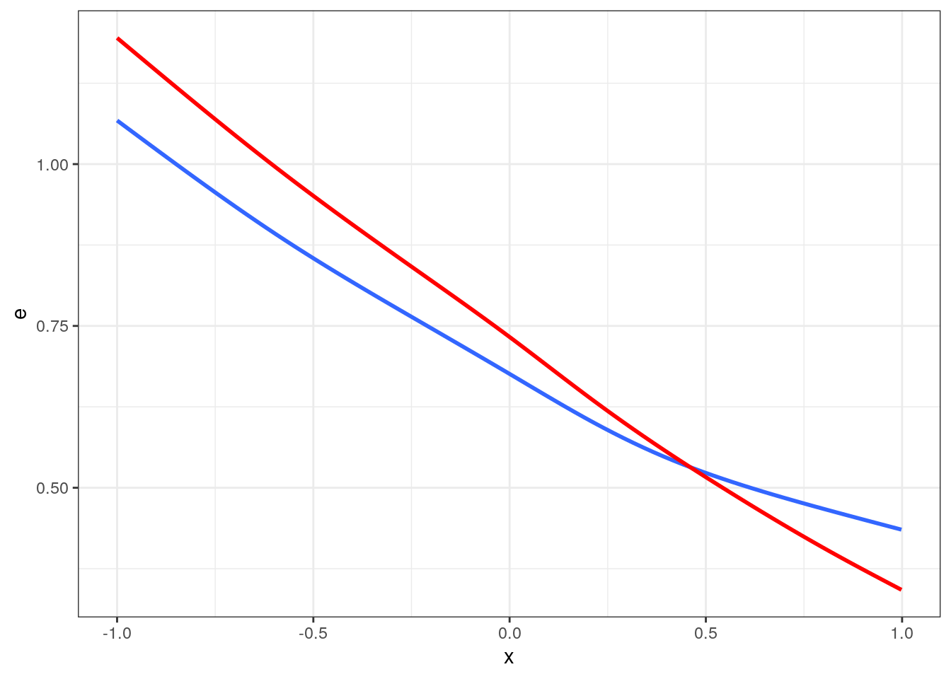

summary(lm(y ~ x + m,data))

## 
## Call:
## lm(formula = y ~ x + m, data = data)
## 
## Residuals:
##     Min      1Q  Median      3Q     Max 
## -3.6919 -0.8389 -0.0532  0.8234  4.5326 
## 
## Coefficients:
##             Estimate Std. Error t value Pr(>|t|)    
## (Intercept) -0.05970    0.07273  -0.821    0.412    
## x            1.11639    0.06001  18.604   <2e-16 ***
## m            1.02399    0.09209  11.119   <2e-16 ***
## ---
## Signif. codes:  0 '***' 0.001 '**' 0.01 '*' 0.05 '.' 0.1 ' ' 1
## 
## Residual standard error: 1.206 on 2493 degrees of freedom
##   (2504 observations deleted due to missingness)
## Multiple R-squared:  0.1225, Adjusted R-squared:  0.1218 
## F-statistic:   174 on 2 and 2493 DF,  p-value: < 2.2e-16

We can see that the regression coefficient is close to it’s true value!

Static Labor Supply