Lab on Discrete Choice
03 January, 2023
- consider estimation of demand model for transport
- look at IIA assumption (potential pitt-falls)
- extend with 3 types, check substitution patterns
- consider max-rank substitution
We consider here discrete choices over a set of alernatives. THe utility of the agent is modeled as
The probit
We consider variables compared to a Normal Distribution.
\[D_i = 1[ X_i \beta + \epsilon_i \geq 0 ]\]
the likelihood for data \((D_i,X_i)\) is given by
\[l_n(\beta) = \sum_i D_i \log \Phi( X_i \beta) + (1-D_i) \log \Big( 1 - \Phi( X_i \beta) \Big) \]
Let’s take simple example:
library(ggplot2)
N = 1000
X = rnorm(N)
beta  = 1.5
E = rnorm(N) # logit instead -> type 1 extreme value
D = X * beta + E >= 0
we then write a likelihood function
lp_n = function(b,D,X) {
  Phi = pnorm(X*b) # pnorm is CDF of N(0,1)
  sum( ifelse(D, log(Phi), log(1-Phi ) ))
  #sum( D*log(Phi) + (1-D) *log(1-Phi ) )
}

lp_n(beta,D,X)
## [1] -398.9191lp_n(beta+1,D,X)## [1] -466.2471lp_n(beta-1,D,X)## [1] -498.3026We then plot this for a grid of beta
lp_vals = unlist(lapply(seq(-1,3,l=100), function(b) lp_n(b, D,X)) )
data = data.frame(beta = seq(-1,3,l=100),lp = lp_vals)

bmax = data$beta[which.max(data$lp)]

ggplot(data,aes(x=beta,y=lp))  + geom_line() +
  geom_vline(xintercept = bmax,linetype=2) +
  geom_vline(xintercept = beta,linetype=3,color="red") +
  theme_bw()
# Running a monte carlo
betas = rep(0,200) #number of replications
N=2000 # sample size

for (r in 1:200) {
  X = rnorm(N)
  beta  = 1.5
  E = rnorm(N)
  D = X * beta + E >= 0

  lp_vals = unlist(lapply(seq(-1,3,l=100), function(b) lp_n(b, D,X)) )
  betas[r] = data$beta[which.max(lp_vals)]
}
ggplot(data.frame(betas = betas),aes(x=betas)) +
geom_histogram(fill="blue", alpha=0.5) +
geom_vline(xintercept = beta,linetype=2,color="red") +
geom_vline(xintercept = mean(betas),linestyle=2,color="green") +
theme_bw()## Warning in geom_vline(xintercept = mean(betas), linestyle = 2, color = "green"):
## Ignoring unknown parameters: `linestyle`## `stat_bin()` using `bins = 30`. Pick better value with `binwidth`.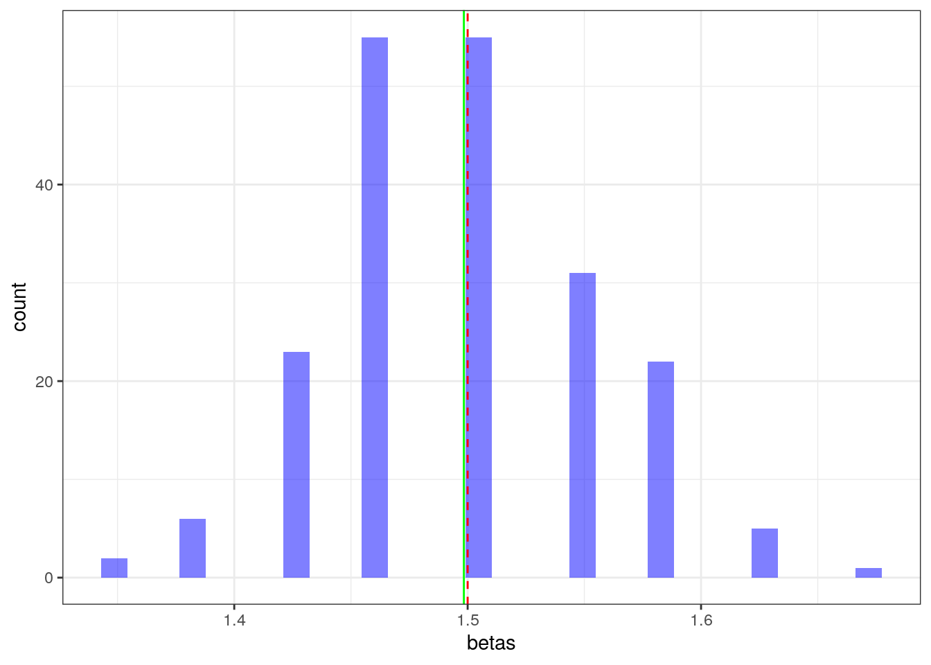
Discrete Choices
Formulate this problem as a pricing problem, like train trying to compete and stragely set prices to maximize profits. It might come together nicely towards the end.
\[u_i(j) = \beta X_i + \epsilon_{ij}\]
and when the error term is type 2 extreme value:
\[F(\epsilon_{ij}) = \exp( -\exp( -\epsilon_{ij} ) )\]
the choice probability is given by
\[ Pr[j(i)^*=j] = \frac{ \exp[ u_i(j) ] }{ \sum_j' \exp[ u_i(j') ]} \]
Armed with these tools we can tackle the data we are given.
Data
library(AER)
library(mlogit)
library(kableExtra)
library(knitr)
library(foreach)
library(ggplot2)
library(data.table)
data("TravelMode")
data = TravelMode

data[1:10,]
## individual mode choice wait vcost travel gcost income size
## 1 1 air no 69 59 100 70 35 1
## 2 1 train no 34 31 372 71 35 1
## 3 1 bus no 35 25 417 70 35 1
## 4 1 car yes 0 10 180 30 35 1
## 5 2 air no 64 58 68 68 30 2
## 6 2 train no 44 31 354 84 30 2
## 7 2 bus no 53 25 399 85 30 2
## 8 2 car yes 0 11 255 50 30 2
## 9 3 air no 69 115 125 129 40 1
## 10 3 train no 34 98 892 195 40 1From the W. Greene Book, chapter 21.7.8:
Hensher and Greene [Greene (1995a)] report estimates of a model of travel mode choice for travel between Sydney and Melbourne, Australia. The data set contains 210 observations on choice among four travel modes, air, train, bus, and car. The attributes used for their example were: choice-specific constants; two choice-specific continuous measures; GC, a measure of the generalized cost of the travel that is equal to the sum of in-vehicle cost, INVC and a wagelike measure times INVT, the amount of time spent traveling; and TTME, the terminal time (zero forcar); and for the choice between air and the other modes, HINC, the household income. A summary of the sample data is given in Table 21.10. The sample is choice based so as to balance it among the four choices—the true population allocation, as shown in the last column of Table 21.10, is dominated by drivers.
Mlogit results
library(AER)
library(mlogit)
library(kableExtra)
library(knitr)
library(reshape2)
data("TravelMode")

TravelMode <- mlogit.data(TravelMode,
                          choice = "choice",
                          shape = "long",
                          alt.var = "mode",
                          chid.var = "individual")
data = TravelMode

## overall proportions for chosen mode
with(data, prop.table(table(mode[choice == TRUE])))
##
## air train bus car
## 0.2761905 0.3000000 0.1428571 0.2809524## travel vs. waiting time for different travel modes
ggplot(data,aes(x=wait, y=travel)) +
geom_point() + facet_wrap(~mode) + theme_bw()## Warning: Combining variables of class <xseries_mlogit> and <factor> was deprecated in ggplot2 3.4.0.
## ℹ Please ensure your variables are compatible before plotting (location: `join_keys()`)
Next we fit a model with cost and wait time as regressors and intercepts for each of the 4 options.
## Greene (2003), Table 21.11, conditional logit model
fit1 <- mlogit(choice ~ gcost + wait, data = data, reflevel = "car")
#fit1 <- mlogit(choice ~ 1 | wait + gcost + income, data = data, reflevel = "car")
# fit1 <- mlogit(choice ~ gcost + wait + income, data = data, reflevel = "car") # why doesn't it work?
summary(fit1)
##
## Call:
## mlogit(formula = choice ~ gcost + wait, data = data, reflevel = "car",
## method = "nr")
##
## Frequencies of alternatives:choice
## car air train bus
## 0.28095 0.27619 0.30000 0.14286
##
## nr method
## 5 iterations, 0h:0m:0s
## g'(-H)^-1g = 0.000221
## successive function values within tolerance limits
##
## Coefficients :
## Estimate Std. Error z-value Pr(>|z|)
## (Intercept):air 5.7763487 0.6559187 8.8065 < 2.2e-16 ***
## (Intercept):train 3.9229948 0.4419936 8.8757 < 2.2e-16 ***
## (Intercept):bus 3.2107314 0.4496528 7.1405 9.301e-13 ***
## gcost -0.0157837 0.0043828 -3.6013 0.0003166 ***
## wait -0.0970904 0.0104351 -9.3042 < 2.2e-16 ***
## ---
## Signif. codes: 0 '***' 0.001 '**' 0.01 '*' 0.05 '.' 0.1 ' ' 1
##
## Log-Likelihood: -199.98
## McFadden R^2: 0.29526
## Likelihood ratio test : chisq = 167.56 (p.value = < 2.22e-16)The intercepts are choice specific, the cost and wait vary accross options and we estimate a common parameter.
We notice that both cost and wait enter negatively. Also air travel seems mostly chosen, indeed it is a long distance.
Predict outcome when changing air price
We want to simulate the demand impact of a price increase for air-travel. And see how people will move from one option to another. We first do this by fixing every alternative to their mean value.
data2 =copy(data)
I=paste(data2$mode)=="air"

# force other alternatives to mean value
for (mm in c('car','train','bus')) {
  data2$gcost[paste(data2$mode)==mm] = mean(data2$gcost[paste(data2$mode)==mm])
  data2$wait[paste(data2$mode)==mm]  = mean(data2$wait[paste(data2$mode)==mm])
}


# run a for lopp for different prices
# save shares for each option
rr = foreach(dprice = seq(-25,25,l=20), .combine = rbind)  %do% {
  data2$gcost[I] = data$gcost[I]*( 1+ 0.01*dprice)
  res = colMeans(predict(fit1,newdata=data2))
  res['dprice'] = dprice
  res
}

rr = melt(data.frame(rr),id.vars = "dprice")
ggplot(rr,aes(x=dprice,y=value,color=factor(variable))) +
  geom_line() + theme_bw() + ggtitle("changing the price of air") + xlab("percent change in price of air") + geom_vline(xintercept = 0, linetype=2)
- this does not include an overall participation margin
- interesting fact that other lines appear to move in parallel!
IIA assumption
Due to the functional form for the multinomial logit, it is the case that the choice of car versus train is not affected by the price of air travel.
This of-course goes away when including some randomness in the covariates and integrating over. Imagine the airline chooses to shift all realized prices, and we then take the average.
data2 =copy(data)
I=paste(data2$mode)=="air"

rr = foreach(dprice = seq(-25,25,l=20), .combine = rbind)  %do% {
  data2$gcost[I] = data$gcost[I]*( 1+ 0.01*dprice)
  res = colMeans(predict(fit1,newdata=data2))
  res['dprice'] = dprice
  res
}

rr = melt(data.frame(rr),id.vars = "dprice")
ggplot(rr,aes(x=dprice,y=value,color=factor(variable))) +
  geom_line() + theme_bw() + ggtitle("changing the price of air") + xlab("percent change in price of air")
Nested logit
One way to test the assumption is to estimate without one alternative
and see if it affects the parameters. For instance we can focus on
whether air or train is chosen and estimate
within.
We then estimate a slightly different distribution. We know allow for choices within groups to have correlated errors within an individual.
TBD math behind the nested logit, show that choices are correlated within nest.
The nest logit, basically models a two stage decision. First one chooses a nest each with associated type I extreme value shocks, then within each nest, the individual chooses the final option. It amounts to sequential decision porcess.
Estimation itself can also be conducted in two stages.
The distribution for a single layer nested logit is
\[ F\left(\vec{\epsilon}_{i t}\right)=\exp \left[-\sum_{r}\left(\sum_{j \in J_{r}} e^{-\frac{\epsilon_{i j t}}{\rho_{r}}}\right)^{\rho_{r}}\right] \]
The \(\rho_r\) parameter controls the level of correlation in draws for choice options in the same \(r\) nest. Larger \(rho\) means less correlation.
We can write:
- \(i\) = alternative, \(k\) = nest, \(n\) = individual, \(1-\lambda_k\) = correlation within branch \(B_k\)
- utility of individual \(i\) from choosing alternative \(i\in B_k\):
\[U_{ni} = W_{nk} + Y_{ni} + \epsilon_{ni}\]
- probability that individual \(i\) chooses alternative \(i\in B_k\):
\[ P_{ni} = P_{ni|B_k} \times P_{nB_k}\\ P_{ni|B_k} = \dfrac{e^{Y_{ni}/\lambda_k}}{\sum\limits_{j\in B_k}e^{Y_{nj}/\lambda_k}}\\ P_{nB_k} = \dfrac{e^{W_{nk}+\lambda_k I_{nk}}}{\sum\limits_{l=1}^K e^{W_{nl}+\lambda_l I_{nl}}}\]
- \(I_{nk}\) = inclusive value:
\[I_{nk} = \ln \sum\limits_{j\in B_k} e^{Y_{nj}/\lambda_k}\]
We can use R to fit a nested logit where we combine the ground transportation inside a given group.
fit.nested <- mlogit(choice ~ wait + gcost, TravelMode, reflevel = "car",
           nests = list(fly = "air", ground = c("train", "bus", "car")),
           unscaled = TRUE)

summary(fit.nested)
##
## Call:
## mlogit(formula = choice ~ wait + gcost, data = TravelMode, reflevel = "car",
## nests = list(fly = "air", ground = c("train", "bus", "car")),
## unscaled = TRUE)
##
## Frequencies of alternatives:choice
## car air train bus
## 0.28095 0.27619 0.30000 0.14286
##
## bfgs method
## 15 iterations, 0h:0m:0s
## g'(-H)^-1g = 6.59E-07
## gradient close to zero
##
## Coefficients :
## Estimate Std. Error z-value Pr(>|z|)
## (Intercept):air 7.0761993 1.1077730 6.3878 1.683e-10 ***
## (Intercept):train 5.0826937 0.6755601 7.5237 5.329e-14 ***
## (Intercept):bus 4.1190138 0.6290292 6.5482 5.823e-11 ***
## wait -0.1134235 0.0118306 -9.5873 < 2.2e-16 ***
## gcost -0.0308887 0.0072559 -4.2571 2.071e-05 ***
## iv:fly 0.6152141 0.1165753 5.2774 1.310e-07 ***
## iv:ground 0.4207342 0.1606367 2.6192 0.008814 **
## ---
## Signif. codes: 0 '***' 0.001 '**' 0.01 '*' 0.05 '.' 0.1 ' ' 1
##
## Log-Likelihood: -195
## McFadden R^2: 0.31281
## Likelihood ratio test : chisq = 177.52 (p.value = < 2.22e-16)In addition to the parameters on the different regressors, this also
returns the Inclusive values iv:fly and
iv:ground which represents the values associated with each
of the nests.
We use the model to simulate price changes and track the impact:
data2 =copy(data)
I=paste(data2$mode)=="bus"

# force other alternatives to mean value
for (mm in c('car','train','air')) {
  #data2$gcost[paste(data2$mode)==mm] = mean(data2$gcost[paste(data2$mode)==mm])
  data2$wait[paste(data2$mode)==mm]  = mean(data2$wait[paste(data2$mode)==mm])
}

# run a for loop for different prices
# save shares for each option
rr = foreach(dprice = seq(-25,25,l=20), .combine = rbind)  %do% {
  data2$gcost[I] = data$gcost[I]*( 1+ 0.01*dprice)
  res = colMeans(predict(fit.nested,newdata=data2))
  res['dprice'] = dprice
  res
}

rr = melt(data.frame(rr),id.vars = "dprice")
ggplot(rr,aes(x=dprice,y=value,color=factor(variable))) +
  geom_line() + theme_bw() +
  ggtitle("changing the price of bus") + xlab("percent change in price of bus")
Random coefficient model
Let’s try with 2 groups of people to run an EM, nee to introduce EM first.
We augment our model with a latent type.
set.seed(6433)

C = acast(data,individual ~ mode,value.var="choice")
C = C[,c(4,1,2,3)]
p1=0.5 # initial guess is both sub-model are equally likely

# we randomly assign 0,1 probability to get starting values
I = sample( unique(data$individual),nrow(data)/8)
I = data$individual %in% I

# we start with the very first mlogit (we randomly sub-sample to create some variation)
fit1 <- mlogit(choice ~ wait +gcost , data = data[I,], reflevel = "car")
fit2 <- mlogit(choice ~ wait +gcost , data = data[!I,], reflevel = "car")

# we have our starting values, we run the EM

# iterate E-step and M-step 15 times
liks = rep(0,15)
for (i in 1:15) {

  # ------ E-STEP ------
  # for each individual we compute the posterior probability given their data
  p1v = predict(fit1,newdata=data)
  p2v = predict(fit2,newdata=data)

  p1v = rowSums(p1v * C)*p1
  p2v = rowSums(p2v * C)*(1-p1)

  liks[i] = sum(log(p1v+p2v))
  #cat(sprintf("ll=%f\n",ll))

  p1v  = p1v/(p1v+p2v)
  p1v  = as.numeric( p1v %x% c(1,1,1,1) )

  # --------- M-STEP --=------
  # finally we run the 2 mlogit with weights
  fit1 <- mlogit(choice ~ wait + gcost , data = data, weights = p1v, reflevel = "car")
  fit2 <- mlogit(choice ~ wait + gcost , data = data, weights = as.numeric(1-p1v), reflevel = "car")

  p1 = mean(p1v)
}
print(fit1)
##
## Call:
## mlogit(formula = choice ~ wait + gcost, data = data, weights = p1v, reflevel = "car", method = "nr")
##
## Coefficients:
## (Intercept):air (Intercept):train (Intercept):bus wait
## 691.094826 363.415853 374.876123 -11.124086
## gcost
## -0.041853print(fit2)##
## Call:
## mlogit(formula = choice ~ wait + gcost, data = data, weights = as.numeric(1 - p1v), reflevel = "car", method = "nr")
##
## Coefficients:
## (Intercept):air (Intercept):train (Intercept):bus wait
## -18.658170 -7.133131 -10.682156 0.304183
## gcost
## -0.043025plot(liks)
Max rank estimator
require(RcppSimpleTensor)## Loading required package: RcppSimpleTensor## Loading required package: Rcpp## Loading required package: inline##
## Attaching package: 'inline'## The following object is masked from 'package:Rcpp':
##
## registerPlugin## Loading required package: digestdata("Train", package = "mlogit")
data = data.table(Train)
fit = glm(choice=="choice1" ~ 0 + I(log(price_A/price_B)) + I(log(time_A/time_B)),data,family = binomial('probit'))
N = nrow(data)
ggplot(data,aes(x=log(price_A/price_B),y=log(time_A/time_B),color=choice)) + geom_point() + theme_bw()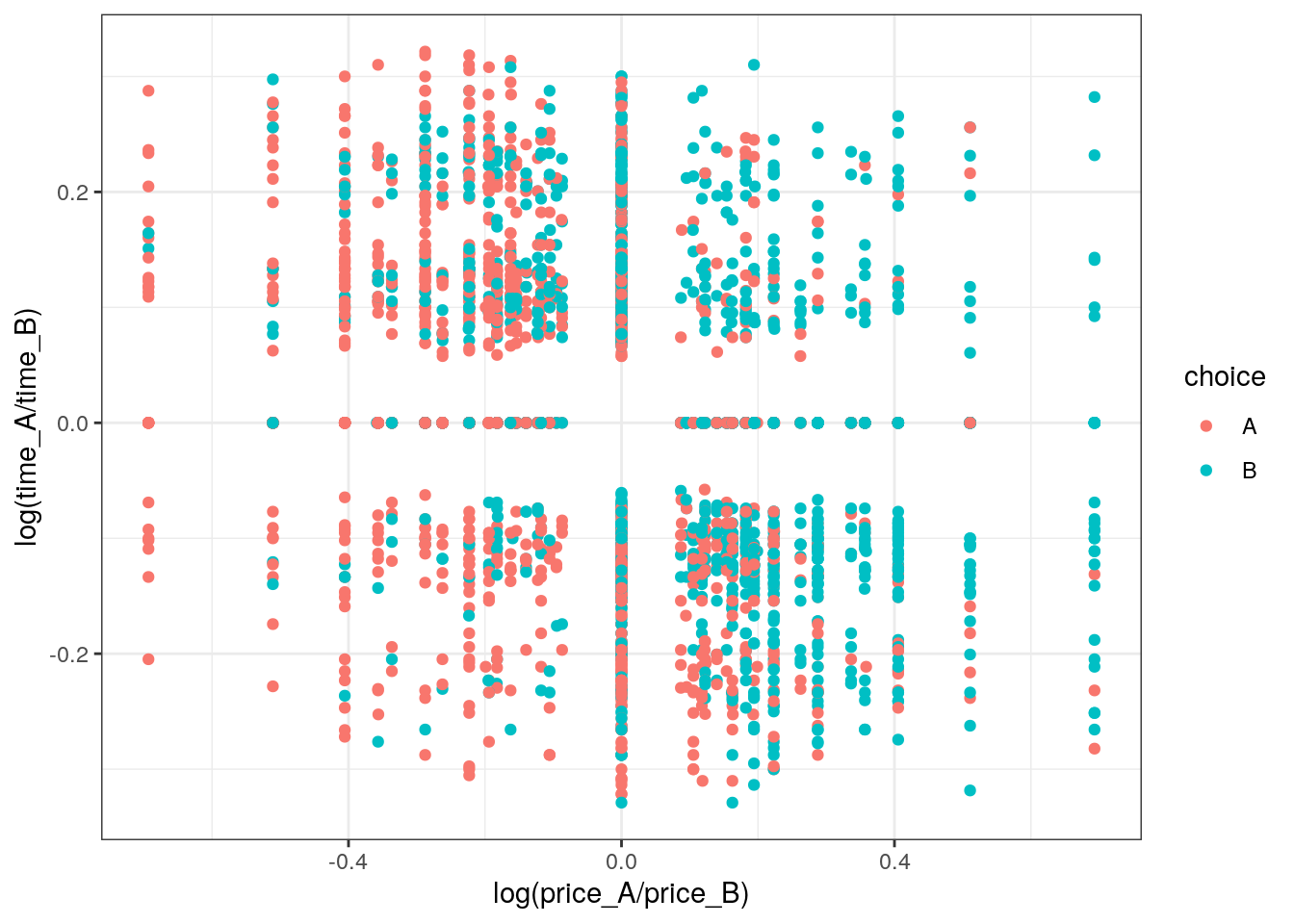
# let's put this in matrices
X = cbind( log(data$price_A/data$price_B), log(data$time_A/data$time_B))
colnames(X) = c("price","time")
Y = (data$choice == "A")*1

t.tmp = tensorFunction(R[i] ~ I(VV[i]<VV[j])*I(Y[i]<Y[j]) + I(VV[i]>VV[j])*I(Y[i]>Y[j]))

# score function
score <- function(beta) {
  tot = 0;
  VV = as.numeric(X %*% beta)
  tot = sum(t.tmp(VV,Y))
  return(data.frame(b1=beta[1],b2=beta[2],val=log(tot)))
}

rr =score(c(0.1,0.1))

require(foreach)
rr = data.table(foreach(b1 = seq(-5,-3,l=40),.combine=rbind) %:%
                  foreach(b2 = seq(-3,-1,l=40),.combine=rbind) %do%
                  score(c(b1,b2)))

library(lattice)
wireframe(val~b1+b2,rr)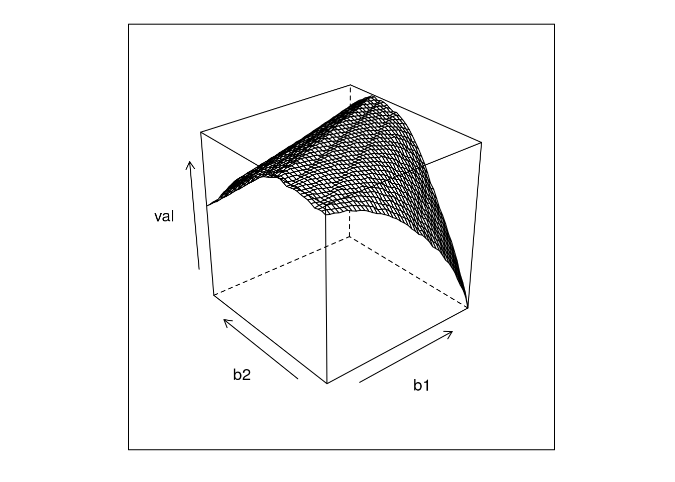
I = which.max(rr$val)
beta_hat = as.numeric(rr[I,c(b1,b2)])
beta     = as.numeric(fit$coefficients)

ggplot(rr,aes(x=b1,y=val,color=b2,group=b2)) + geom_line() +theme_bw() +
  geom_vline(xintercept = beta[1],color="red",linetype=2) +
  geom_vline(xintercept = beta_hat[1],color="blue",linetype=2)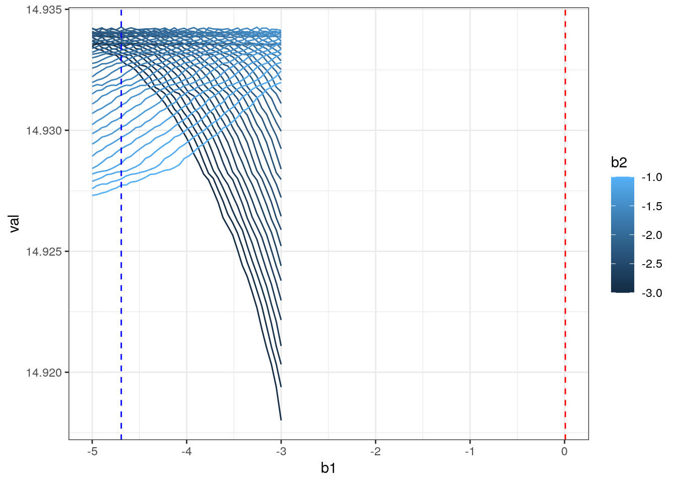
ggplot(rr,aes(x=b2,y=val,color=b1,group=b1)) + geom_line() +theme_bw() +
  geom_vline(xintercept = beta[2],color="red",linetype=2) +
  geom_vline(xintercept = beta_hat[2],color="blue",linetype=2)
#fit2 <- mlogit(choice ~ price + time + change + comfort |-1, Tr)Recovering the distribution of unbosverables:
dd = data.table(Y=Y,R_hat= as.numeric(X%*%beta_hat))
g <- function(x0,h) dd[, sum( Y * dnorm( (R_hat-x0)/h))/sum( dnorm( (R_hat-x0)/h)) ]
h=0.3
dd = dd[, F_hat := g(R_hat,h),R_hat]

ggplot(dd,aes(x=R_hat,y=F_hat)) + geom_line(color="red")  + theme_bw() +
  geom_line(aes(x=R_hat,y=plogis(R_hat)),color="blue",linetype=2) +
  geom_line(aes(x=R_hat,y=pnorm(R_hat)),color="green",linetype=2)